How to Train Graph Neural Networks: From First Principles to Planet Scale

A 3-layer GNN training on 111 million nodes produces 336 gigabytes of intermediate data. The best GPU cluster you can buy has 320 gigabytes of memory. The training run crashes before the second epoch.

That crash is not a hardware problem. It is a planning problem.

This article is a companion to the Irys University video of the same name. It covers the same ground in written form: why graphs are the right representation for many real-world problems, how GNNs learn from graph structure, why full-graph training is essential for correctness, and how FlexGNN solved the memory wall by reframing GPU capacity from a hard limit into an optimization variable.

Part I: Why Graphs Matter

The World Is a Graph

Social networks, molecular structures, supply chains, power grids, financial transaction networks, legal citation graphs. Every one of these domains shares the same mathematical shape: nodes connected by edges, where the connections carry information that tabular records cannot.

A fraud detection system built on transaction tables sees individual transfers. A graph-based system sees the layering pattern: one account fans out to three intermediaries, which fan back into one aggregator, which converts to foreign exchange. The individual transactions are each unremarkable. The shape of the graph is the signal.

GraphCast, DeepMind's weather prediction model, treats Earth's atmosphere as a graph where each spatial location is a node and physical interactions define edges. It beat the gold-standard ECMWF HRES forecast on 90% of evaluation targets. GNoME discovered 2.2 million new stable crystal structures by training on molecular graphs. In both cases, full-graph training was not optional. Sampling the graph broke the physics.

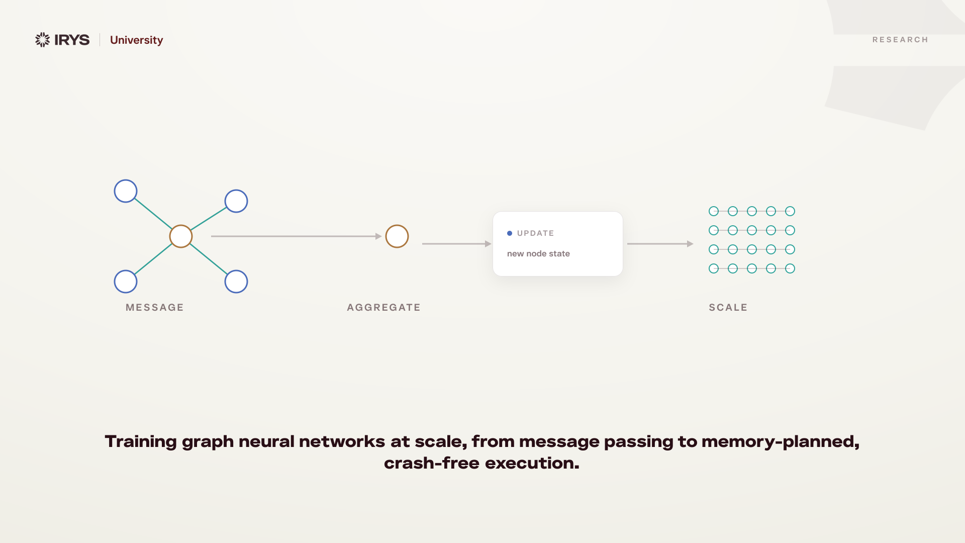
Message Passing

GNNs learn through message passing. Each node collects feature vectors from its neighbors, aggregates them (typically by averaging or summing), combines the aggregate with its own features, and passes the result through a learned transformation.

One layer of message passing lets each node see its immediate neighbors. Two layers lets it see neighbors-of-neighbors. Three layers gives a 3-hop receptive field. This is how local structure becomes global understanding.

Graph Attention Networks (GAT) refine this by learning attention weights on each edge. Instead of treating all neighbors equally, the model learns which connections matter more for the task at hand.

The Memory Problem

Each layer of message passing stores intermediate activations for backpropagation. The chain rule requires forward-pass values to compute gradients during the backward pass.

For a standard neural network, intermediate storage scales with batch size times number of layers. For a GNN, it scales with nodes times layers times feature dimension. On a graph with 111 million nodes and 3 layers, that is 336 GB of intermediate data.

The neighborhood explosion makes it worse. Each additional layer multiplies the number of neighbors a node must aggregate. On a degree-10 graph, layer 1 touches 10 neighbors. Layer 2 touches 100. Layer 3 touches 1,000. Memory grows exponentially with depth.

Sampling Is Not the Answer

GraphSAGE and related methods reduce memory by sampling a fixed number of neighbors per layer. This works for some applications, but it introduces four forms of damage:

• Structural damage. Connectivity patterns are lost.
• Gradient bias. Gradient estimates become biased.
• Convergence delay. More epochs are needed to compensate.
• Accuracy loss. Final performance is lower than full-graph training.

For weather prediction, materials science, and fraud detection, sampling is unacceptable. The physics, chemistry, or pattern recognition depends on the complete graph structure.

Part II: Why Full-Graph Training Crashes

Backpropagation Stores Everything

During the forward pass, every layer's output is stored in GPU memory because the backward pass needs those values to compute gradients. This is not a design choice. It is a mathematical requirement of gradient-based optimization.

GNN intermediates are particularly expensive because they scale with graph size, not batch size. A transformer training on batch size 32 stores 32 copies of each layer's activations. A GNN training on a 111-million-node graph stores 111 million copies.

The Memory Hierarchy

Modern GPU systems have three tiers of storage:

• HBM (GPU). Capacity around 80 GB on an A100. Bandwidth around 2,039 GB/s. Think of it as the penthouse.
• Host RAM. Capacity from 512 GB to 2 TB. Bandwidth around 64 to 128 GB/s over PCIe. Think of it as the warehouse.
• SSD. Capacity at the terabyte scale. Bandwidth around 14 GB/s over NVMe. Think of it as the ocean floor.

The bandwidth gap is enormous. HBM is 26 times faster than PCIe on an A100, and 240 times faster than NVMe SSD. Moving data between tiers is expensive. But the lower tiers have vastly more capacity.

Multi-GPU training adds NVLink (600 GB/s on A100), which lets GPUs communicate directly. But exchange buffers for multi-GPU communication consume additional GPU memory, creating a secondary pressure on the scarce HBM tier.

Prior Art and Its Limits

The field has tried two approaches, both with significant limitations.

Sampling camp: Sancus (Skip-Broadcast) achieves 74% communication reduction but runs out of memory at 16 nodes. BNS-GCN (Boundary Node Sampling) achieves 99% communication reduction but spends 97% of remaining time on communication overhead.

Full-graph camp: ROC uses dynamic programming for memory management but lacks latency hiding. HongTu (SIGMOD 2024) introduced 2-level partitioning and is the most sophisticated pre-FlexGNN system, but uses only static recomputation. NeutronStar attempts CPU-GPU collaboration but runs out of memory on ogbn-papers and friendster.

No prior system combines adaptive communication, dynamic memory planning, latency hiding, and SSD-tier integration.

Part III: FlexGNN, The Paradigm Shift

Memory as Optimization Variable

FlexGNN reframes the question. Instead of asking "does it fit?" (which has a binary answer that ends in a crash), it asks "what is the cheapest plan?" (which always has a solution).

The key insight: GPU memory is not a wall. It is an optimization variable. The planner profiles the hardware (GPU memory, host RAM, SSD capacity, bandwidth at every tier) and the model (operator graph, activation sizes, dependency chain), then computes an optimal execution plan before training begins.

The Four Fates

Every intermediate datum produced during the forward pass must eventually be available for the backward pass. FlexGNN recognizes four legal fates for each datum:

• Retain on GPU. Zero time cost. GPU memory cost is the datum size divided across the GPUs. No host memory cost.
• Offload to host RAM. Time cost is two PCIe transfers, the size of the datum each way. No GPU memory cost. Host memory cost is the datum size.
• Offload to SSD. Time cost is two round trips adjusted for latency hiding. No GPU memory cost. No host memory cost.
• Recompute. Time cost is the cost of re-executing the forward operator. No GPU memory cost. No host memory cost.

Retention is fastest but consumes scarce HBM. Host offloading frees GPU memory but costs two PCIe transfers (offload plus reload). SSD offloading is the slowest transfer but frees both GPU and host memory. Recomputation costs zero memory but requires re-executing the forward operator.

The optimal plan depends on the specific hardware configuration, graph size, model architecture, and available memory at each tier.

Dynamic Programming for Fate Assignment

Choosing the cheapest combination of fates is a global optimization problem. Retaining one large datum might force five others to be offloaded. Recomputing one expensive operator might free enough memory to retain three cheap ones.

FlexGNN solves this with dynamic programming. For each intermediate datum, the dynamic program evaluates all four fates while respecting memory budgets at every tier. The result is a globally optimal assignment that minimizes total execution time subject to memory constraints.

Key concepts in the formulation:

• Lifetime intervals. Each datum has three critical points: when it is produced (forward), when it is last used (forward), and when it is needed again (backward). The interval between last forward use and backward reuse defines the window for offloading or recomputation.
• Memory budgets. The GPU memory budget and host memory budget are constraints that the dynamic program must satisfy at every point in time.
• Latency hiding. Transfers can overlap with computation. A latency-hiding factor captures what fraction of transfer time is hidden behind useful compute. A higher factor means offloading is cheaper than it appears.

Operator Scheduling

After fates are assigned, FlexGNN schedules the actual operations: when to offload each datum, when to reload it, and how to interleave transfers with computation to maximize latency hiding.

The scheduling respects three constraints:

• Offload only after the datum's last forward use.
• Reload before the datum's backward need.
• Respect bandwidth limits at each tier.

The result is a Gantt chart of operations where compute and transfers overlap, bandwidth is fully utilized, and memory constraints are satisfied at every time step.

Adaptive Communication

Multi-GPU GNN training requires boundary node communication. Prior systems chose either GPU-to-GPU (G2G, fast but memory-hungry for buffers) or GPU-to-Host-to-GPU (G2H, no buffer overhead but slow).

FlexGNN evaluates both strategies per layer and switches adaptively. When GPU memory is abundant, it uses G2G for speed. When memory is tight, it switches to G2H to avoid running out of memory. Unified exchange buffers serve both strategies, eliminating wasted memory.

Part IV: Evidence

Benchmark Results

FlexGNN was evaluated on five benchmark datasets spanning four orders of magnitude in graph size:

• reddit. 233K nodes. FlexGNN speedup of 1.2x.
• ogbn-products. 2.4M nodes. FlexGNN speedup of 2.8x.
• it-2004. 41M nodes. FlexGNN speedup of 4.1x.
• ogbn-papers. 111M nodes. FlexGNN speedup of 4.9x.
• igb260m. 269M nodes. FlexGNN speedup of 5.6x.

The advantage grows with graph size. On small graphs where everything fits in GPU memory, FlexGNN matches existing systems. On large graphs where prior systems crash, FlexGNN runs to completion and achieves substantial speedups.

On the out-of-memory test, FlexGNN completed all five benchmarks. HongTu failed on igb260m. NeutronStar failed on ogbn-papers and igb260m. Sancus failed on it-2004 and larger.

The planner generates execution plans automatically. No manual tuning is required. The same planner works across GPU generations and graph sizes.

Part V: Implications

The Execution Planner Thesis

FlexGNN's four fates and dynamic-programming planning are not specific to GNNs. They apply to any computation with:

• A directed acyclic graph of operators
• Intermediate data between operators
• A memory hierarchy with different capacity and bandwidth tradeoffs

Transformers. Attention produces intermediates that scale with the square of the sequence length. Feed-forward activations scale with sequence length times model dimension. The KV cache grows with layers times sequence length. Current solutions (gradient checkpointing, ZeRO, ad-hoc activation offloading) are manual and fragmented. FlexGNN-style planning could unify them.

Diffusion models. A thousand denoising steps through a U-Net, each storing activations. Total intermediate storage can reach 10 to 100 times the base model size.

Mixture of Experts. Expert parameters are rarely active simultaneously. A planner could offload idle experts to host RAM or SSD and retain only the active ones on GPU.

KV Cache management. Long-context inference (128K or more tokens) produces KV caches that exceed GPU memory. A planner could retain hot layers, offload warm layers to host RAM, and recompute or SSD-offload cold layers.

Planners as the Next CUDA

CUDA abstracted GPU hardware. Execution planners abstract memory management. The developer specifies what to compute. The planner decides where data lives and when it moves.

The abstraction stack:

• Application. Define model and data.
• Execution Planner. Optimize memory layout and operation schedule.
• Runtime. Orchestrate GPU, host, and SSD.
• Hardware. GPU plus NVLink plus PCIe plus SSD.

Before CUDA, engineers hand-tuned GPU kernels. After CUDA, they wrote code and compiled it. Before execution planners, engineers hand-tuned memory management. After execution planners, they profile, plan, and execute.

The Irys Parallel

Irys operates in the legal domain, where the resource hierarchy is knowledge rather than memory. Context windows are scarce and fast. Retrieved documents are abundant but slower. Derived reasoning is unlimited but expensive.

The planning parallel is direct:

• Retain on GPU maps to keeping work in active context.
• Offload to host maps to retrieving from the knowledge base.
• Offload to SSD maps to archiving with metadata.
• Recompute maps to deriving from first principles.

Both systems share the same core insight: planning beats brute force. Adapting to the resource hierarchy, rather than treating it as a wall, turns impossible workloads into routine operations on the same hardware.

Closing

FlexGNN turned a 269-million-node GNN training from impossible to routine on four GPUs. No new chips. No larger servers. Just a better plan.

The memory wall that blocks GNN training at scale blocks every large AI workload. Transformers, diffusion models, mixture-of-experts, long-context inference. Each hits the same constraint: intermediate data exceeds GPU memory.

The question is no longer whether full-scale training is possible. FlexGNN answered that.

The question is who plans it best.

This article accompanies the Irys University video "How to Train Graph Neural Networks: From First Principles to Planet Scale." For the full two-hour visual walkthrough, see the Irys University channel.

Published by Irys AI, planned intelligence for legal work.