How Fractals Can Improve How AI Models Internally Represent Information
A deep dive into hierarchy and why present AI systems are missing it.
When you chop an embedding from 256 dimensions down to 64, what should happen to the meaning?
The entire industry — from the Matryoshka papers to the latest vector database optimizations — treats this as a compression question; truncating embeddings is like 1080p to 360p. You get a blurrier version of the same thing.
But that’s a stupid way to do things. And today we’re going to prove why.
Dimensional truncation in current embeddings is informationally degenerate. It implicitly treats embedding dimensions as a flat bucket of capacity. We assume that dimension #42 and dimension #255 contribute equally to meaning. But meaning isn’t flat. It’s hierarchical. A document about “The Capital of France” is simultaneously about Geography (coarse), Europe (medium), and Paris (fine).
Current embeddings smear these levels across the entire vector. To know the coarse topic, you have to read the fine dimensions. To know the fine details, you have to read the coarse dimensions. This is an access-complexity penalty that forces you to pay full compute costs for simple questions. It also makes auditability a nightmare and makes things like AI re-learning very difficult. In this article, we will present a better way to do this.
Starting from first principles, we leveraged successive refinement theory to pinpoint exactly how embeddings should allocate information hierarchically across dimensions. The theory gave us four precise, falsifiable predictions. We ran the experiments — every single one confirmed. By aligning dimensional truncation with hierarchical meaning, we unlock an infrastructure-level efficiency leap, available immediately at zero additional inference cost.
In this article, we will cover:
What embeddings actually are — and why flat supervision is structurally wasteful.
The information-theoretic argument for hierarchy-aligned rate allocation.
The four causal ablations that isolate alignment as the mechanism.
The scaling law that predicts when and how much this works.
The engineering reality: zero inference cost, measurable retrieval gains.
The broader implication: why information theory still has unfinished business in modern representation learning.
This and much of our research is driven by one manifesto: AI should be like electricity. It should be like vaccines. It should be cheap, ubiquitous, and useful to the poorest person on the street, not just the richest corporation in the cloud. To be a tool that uplifts everyone, instead of concentrating value in the tech oligarchy and their investment bankers.
When we use first-principles analysis to map the structure of thought, we aren’t just doing math. We are finding the efficiency arbitrage that allows us to run powerful intelligence on cheap hardware, making intelligence more accessible to everyone. Consequently, there will be more math than most of you signed up for, but I’m going to trust in your intelligence to follow along. This work has implications that go far beyond embeddings (we’re exploring the upper limits of what LLMs can and can’t encode in their information and working to fix that), and thus we need to pay the foundations their due respect.

I also recognize that we will make some extremely bold claims of performance and results in this article. Therefore, I am sharing EVERYTHING we’ve found in this state on this GitHub repo. There you will find the intermediate data, code to reproduce experiments, analysis, longer theoretical discussions, and more. I encourage you to check my work, tell me where you see gaps, and work on it with me so we can ensure that the future of intelligence stays open source(we will keep updating the repo with more experiments, so star it to follow along if you’re interested).
So, my valentines, get ready to slide with me as we spread these sheaves and show love to the curves belonging to the geometry of intelligence.
Executive Highlights (tl;dr of the article)
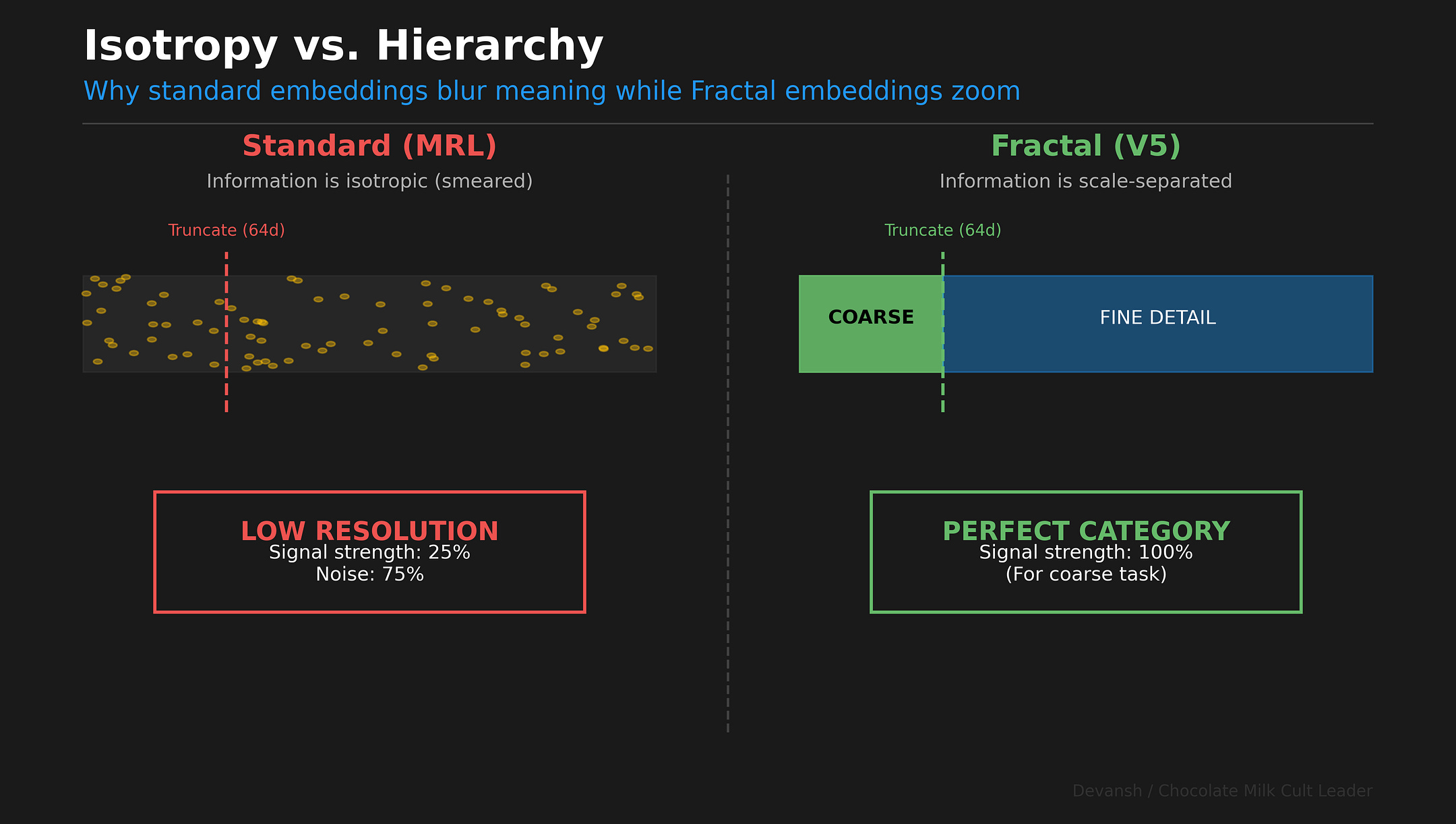
When you truncate an embedding from 256 dimensions to 64, what changes?
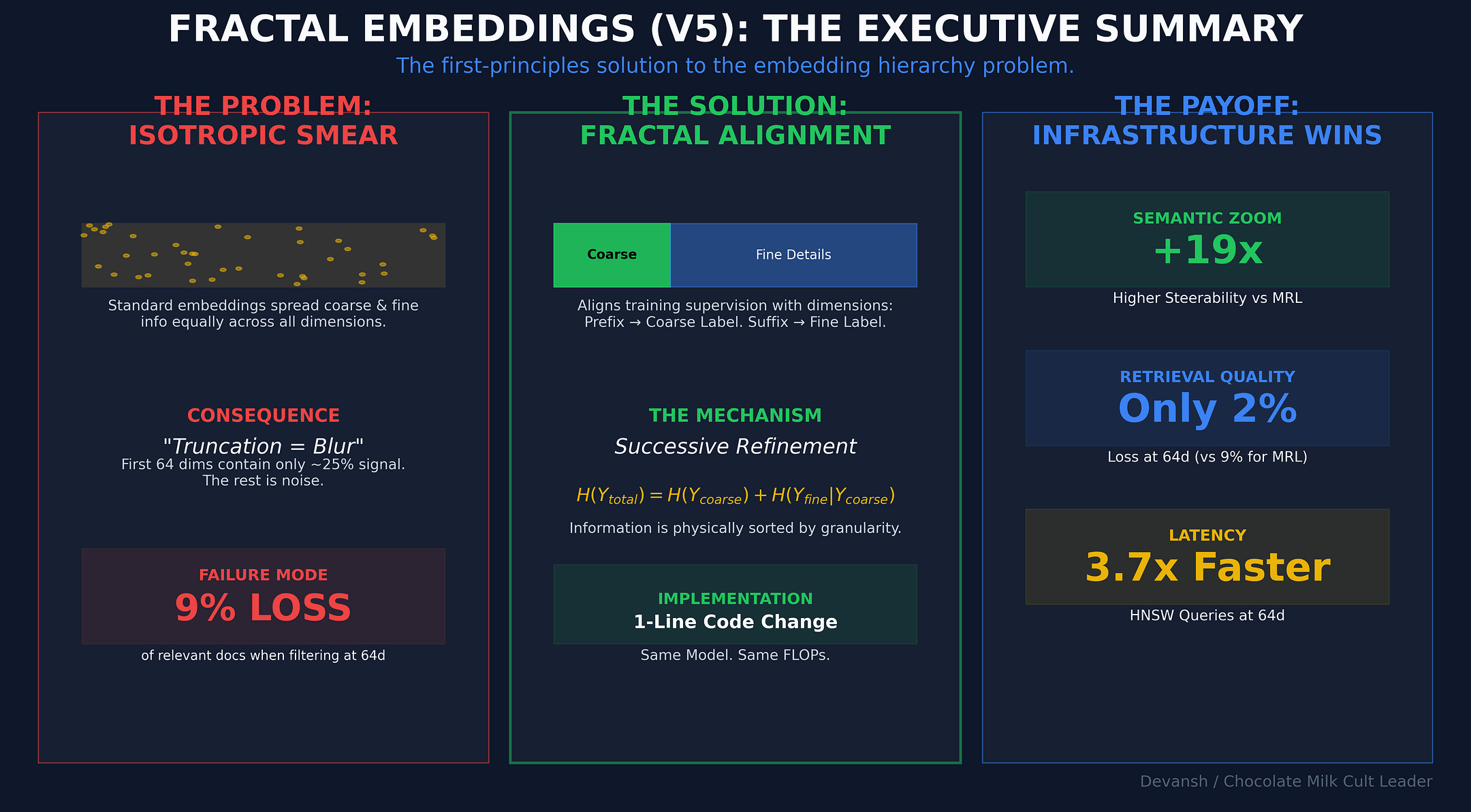
In standard training (MRL), nothing structural changes. You just get a blurrier version of the same meaning. Every prefix is trained on the fine label, so information gets smeared across the whole vector. Read 25% of the dimensions, you get 25% of everything. That’s why you can’t use the first 64 dimensions as a clean “coarse filter.” They’re just low-resolution noise.
But meaning isn’t flat. It’s hierarchical. Every fine label sits inside a coarse label. And information theory tells us something very simple:
total information = coarse bits + refinement bits.
If that’s true, then an embedding shouldn’t treat all dimensions equally. The early dimensions should carry the coarse information. The later ones should refine it. That’s successive refinement.
So we changed one thing: short prefixes are supervised on coarse labels, full embeddings on fine labels. Same architecture. Same parameters. Same inference cost. Just a different training signal.
From that, four predictions fall out:
If alignment drives the effect, then aligned supervision should produce positive steerability.
If we flip the supervision, the sign should flip.
If we make the model “aware” of hierarchy but don’t align prefixes to levels, the effect should collapse.
And there should be a Goldilocks point where prefix capacity matches coarse entropy.
We ran all four. All 4 gave us amazing validation
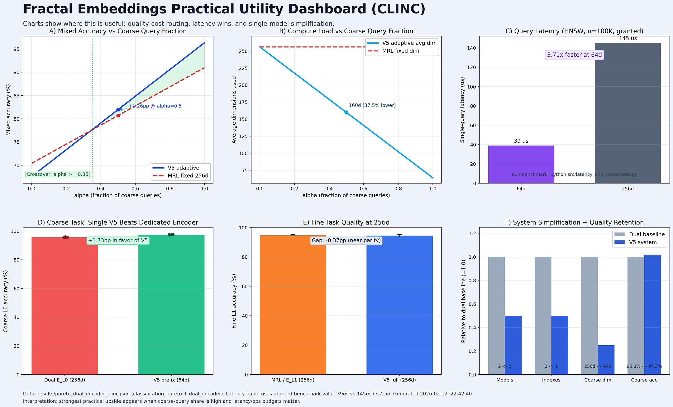
In production, this costs nothing extra. Same embedding size. Same FLOPs. But retrieval behaves differently. On CLINC, V5 shows a +6.3pp recall ramp from 64d to 256d; MRL barely moves. At 64d, HNSW queries are ~3.7× faster. V5 enables meaningful coarse-to-fine routing. MRL truncation mostly doesn’t.
This opens up several efficiency gains, and provides us further validation that there is a whole frontier of performance we can reach through algorithmic gains and efficiency, not scale. We will continue to release more research that proves this.

I provide various consulting and advisory services. If you‘d like to explore how we can work together, reach out to me through any of my socials over here or reply to this email.
SECTION 1: A Gawaar’s Introduction to Embeddings
To really get on the same page, let’s take one second to really define our terms.
1a. The Encoding Problem
Every modern AI system encodes knowledge by embedding concepts — words, tokens, or higher-order abstractions — into vectors. Each vector is a point in a high-dimensional space. Distances and angles between these points define the semantic structure of the model’s world: words that are closer are considered related, directions correspond to relationships, and clusters capture categories. The angle between the vectors for “king” and “queen” mirrors the angle between “man” and “woman.” This is how models “reason.”
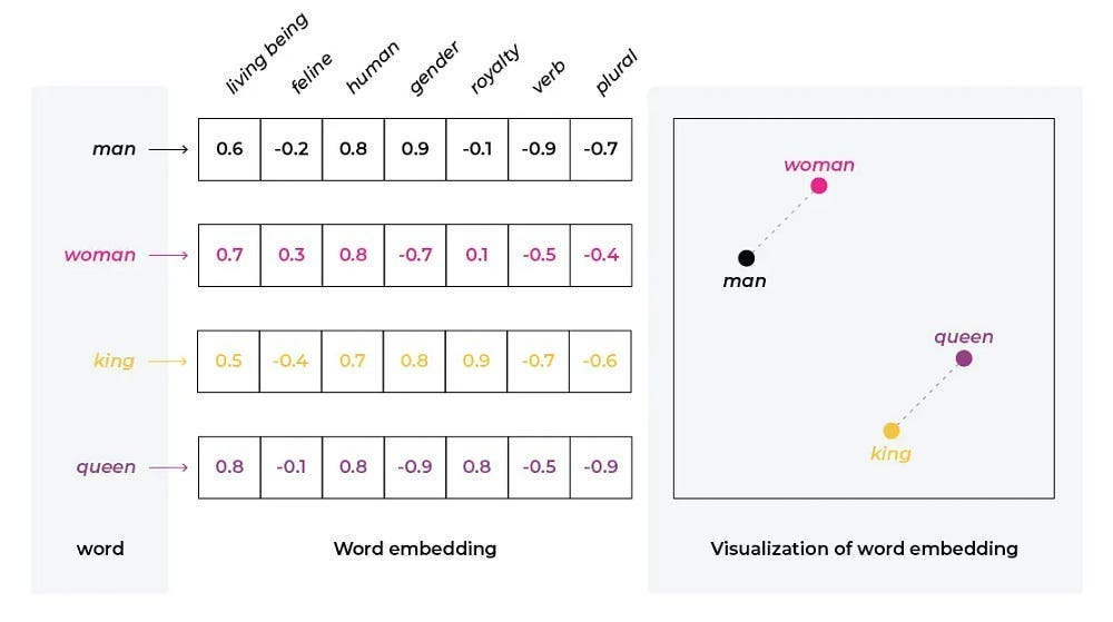
But this space is not cleanly partitioned. For efficiency, models layer thousands of different features into the same vector. This is superposition: a single coordinate encodes multiple, overlapping meanings. Superposition is the reason embeddings are so powerful, but also why they are so opaque. The representation is dense and information-rich, but for humans, almost unreadable.
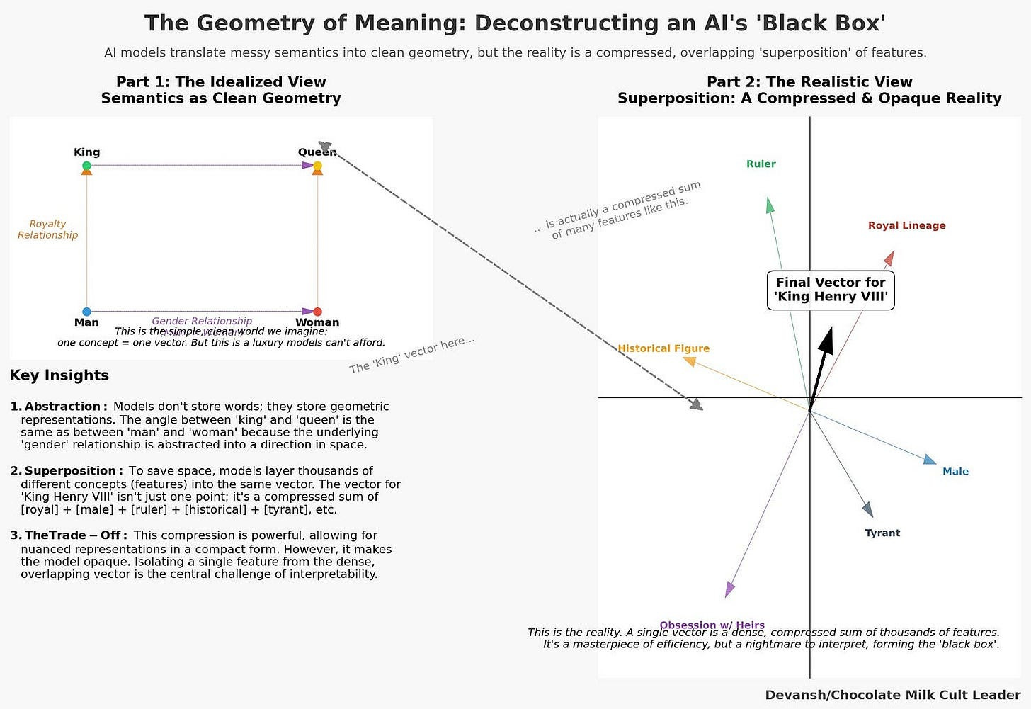
To make AI safe, to underwrite its decisions, to trust it with anything that matters, we must reverse this process. We have to break the superposition. We must find the “atomic basis” — the dictionary of pure, monosemantic features — that the model uses to construct its world.
We’ve already spoken at length about superpositions and why they’re such an important aspect of AI research over here, so we won’t get back into that for this article. For our purposes, it’s important to simply note how encodings work and why superposition creates problems. Our work will address one of the biggest limitations that our current paradigm has.
1b. The Hierarchy Problem Nobody Talks About
Let’s pull up our query: “What is the capital of France?” again. This query carries information at multiple scales simultaneously:
Level 0 (Coarse): It is a GEOGRAPHY question.
Level 1 (Fine): It is about FRANCE.
Level 2 (Finer): It is asking for a CITY.
Every real-world classification system — from library decimal codes to e-commerce product trees to biological taxonomies — is similarly hierarchical. And yet, the vectors we use to represent this meaning are flat.
In a standard embedding of 1024 dimensions, dimension #42 and dimension #900 perform the exact same job. They both try to capture “Geography” and “France” and “City” all at once. The information is smeared across the entire array like jam on toast.
This is called isotropy: every direction in the vector space behaves the same way (embeddings don’t turn out to be isotropic in practice, but that is an assumption you make when you develop things this way; that’s one reason embeddings are a mess to improve since their nature and development conflict with each other).
1c. Why This Matters Economically
This structural mismatch creates a massive economic inefficiency in the vector search market. Our cost can be modeled as
Cost= Number of Documents (N) * Dimensions (D)
If you are running a search for “running shoes” on an e-commerce site, the first thing you need to know is that the user isn’t looking for “kitchen appliances.” That is a coarse, Level 0 distinction.
Retrieval compute is where it gets real. Each query at 256d requires 256 multiply-accumulate operations per candidate vector. At 64d, it’s 64. For a brute-force scan over 100M vectors at 500M queries/day, switching coarse queries (say 250M/day) from 256d to 64d saves roughly~111 trillion FLOP/s of sustained throughput. On approximate nearest neighbor indexes (HNSW, IVF), the savings are smaller in absolute FLOPS but the latency improvement is direct: our benchmarks show 3.7x faster queries at 64d vs 256d on HNSW with 100K vectors.
In an ideal world, you would extend this further to look at the first 64 dimensions of the vector, realize “Oh, this is Sports,” and stop processing the “Appliances” section of your database. You would pay 25% of the compute cost to filter out 90% of the wrong answers.
But you can’t do that today.
Because standard embeddings are often desgined like they’re isotropic, the first 64 dimensions don’t give you the category cleanly. They give you a low-resolution, noisy version of the specific query. They are just as likely to confuse “running shoes” with “running a business” because the semantic resolution is too low.

To get the category right, current models force you to compute the full 1024 dimensions. You are paying for high-definition fidelity when you only need a low-definition filter.
This leads to our core question of the day: Is this smear inevitable? Is the “flatness” of embeddings a fundamental property of neural networks, or is it just a training bug we’ve all accepted as fact?
The math says it’s a bug.
SECTION 2: Three Theorems Beefing with Every Embedding You’ve Ever Used
The way Generative AI represents knowledge and links concepts is flawed and stupid. And I’m going to use math to prove it.
2a. Defining our Terms
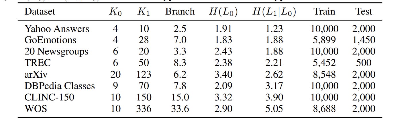
We have fine labels Y₁ (150 specific intents like “book_flight,” “cancel_order”) that nest cleanly inside coarse labels Y₀ (10 domains like TRAVEL, SHOPPING). Every fine label maps to exactly one coarse label. No ambiguity (real knowledge work has composite labels, which we will go deeper into future breakdowns and experiments; this is simply the start of a great lifelong commitment together).
Our embedding vector z gets split into 4 equal blocks: z = [z₁ ; z₂ ; z₃ ; z₄]. Each block is 64 dimensions if the full embedding is 256d. The “prefix” z≤m is just the first m blocks.
The question: can we train z so that z≤1 (64d) reliably encodes the coarse label, and the full z (256d) encodes the fine label?
2b. Theorem 1: The Flat Tax Problem
Standard training applies the same objective to every prefix length: predict the fine label. MRL does exactly this. All prefixes target Y₁.
So there’s no structural pressure for the first 64 dimensions to carry coarse information specifically. The optimizer has no reason to put GEOGRAPHY in dimensions 1–64 and FRANCE in dimensions 65–128. It spreads everything everywhere, because that’s what uniform objectives incentivize.
More mathematically, under an isotropic embedding, signal for any hierarchy level is distributed uniformly across all D dimensions. If you truncate to m dimensions, the signal you observe scales as m/D. Read 64 out of 256 dimensions, get 25% of the signal for everything. Coarse and fine alike. This is the access-complexity penalty — truncation can’t selectively access coarse information. It just gets a quarter of all the information. Useless for routing.
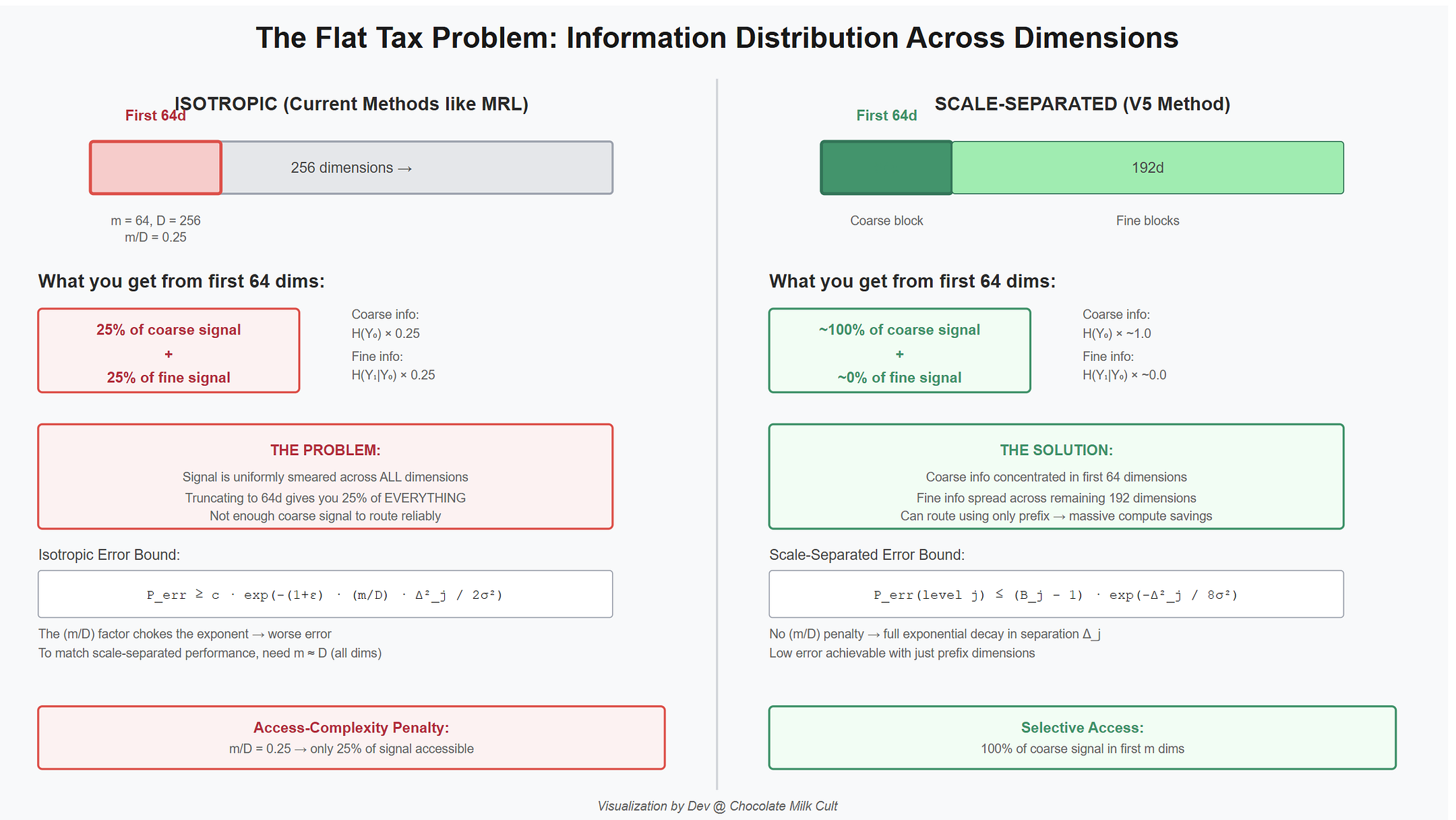
A scale-separated embedding concentrates coarse information in the first block. Reading 64 dimensions gives you nearly 100% of the coarse signal. That’s zoom, not blur.
Let’s make this precise. Imagine your embedding f(x) has Gaussian noise: Y = f(x) + Z, where Z ~ N(0, σ²I). The noise represents everything that makes real embeddings imperfect — finite data, optimization noise, messy language. You want to classify which coarse class a sample belongs to by reading only the first m dimensions.
The scale-separated bound (the good case):
P_err ≤ (B − 1) · exp(−Δ² / 8σ²)
Where each term comes from:
P_err — the probability you classify the coarse label wrong using only the prefix dimensions.
(B − 1) — the number of wrong coarse classes you could be confused with. If there are B = 10 domains, there are 9 wrong answers. This is a union bound: the probability of any mistake is at most the sum of each pairwise mistake. More classes = more chances to screw up. Just counting.
Δ — the minimum distance between any two coarse-class centroids in the prefix subspace. How far apart the clusters sit. Larger Δ = easier to tell apart.
Δ² / 8σ² — this needs unpacking. Two coarse-class centroids sit Δ apart. The decision boundary is the midpoint — equidistant from both. So to get misclassified, noise has to push your point Δ/2 away from its true centroid, past the midpoint, toward the wrong one. Now: how likely is that? The Gaussian bell curve drops off as exp(−distance² / 2σ²). The distance the noise needs to cover is Δ/2. So you square it: (Δ/2)² = Δ²/4. Divide by 2σ²: you get Δ² / (4 · 2σ²) = Δ² / 8σ². That’s where the 8 comes from. It’s just the geometry of “halfway between two points” combined with the Gaussian tail formula.
exp(−...) — the error decays exponentially as separation increases relative to noise. Doubling Δ gives quadratically better protection (because Δ is squared). Doubling σ gives quadratically worse protection.
The critical thing: m doesn’t appear in this bound. The number of prefix dimensions isn’t in the formula. As long as the coarse centroids are well-separated within the prefix subspace, the prefix alone is sufficient. The scale-separated structure put all the relevant signal where you’re looking.
The isotropic bound (the bad case):
P_err ≥ c · exp(−(1+ε) · (m/D) · Δ² / 2σ²)
Term by term:
P_err — same as above, coarse classification error using m truncated dimensions.
c — a constant from the specific hard distribution. This is a lower bound — it says there exists a distribution where you cannot do better than this. Not worst case hand-waving; a proven floor.
(m/D) — this is the entire story. In an isotropic embedding, coarse information is spread uniformly across all D dimensions. You’re reading m of them. Each dimension carries the same fraction of the signal, so m dimensions carry (m/D) of the total squared separation. Why squared? Because separation is a distance — it’s the square root of summed squared per-dimension contributions. If all D dimensions contribute equally to Δ², then m dimensions contribute (m/D) · Δ², and that (m/D) ends up inside the exponent. At m = 64, D = 256: this factor is 0.25. That’s not “25% worse.” It’s exponentially worse because it’s multiplying the exponent. exp(−0.25x) vs exp(−x) is a catastrophic gap for any meaningful x.
(1+ε) — a small technical correction factor for the formal proof. Close to 1. Ignore for intuition.
Δ² / 2σ² — separation vs. noise, same physics as before. The slightly different constant (2 vs 8) comes from this being a lower bound via a different proof technique, not from different physics.
Why this gap is devastating:
The scale-separated embedding’s error depends on Δ in the prefix subspace — a quantity it can optimize during training, concentrating coarse signal exactly where you’ll look. The isotropic embedding’s error is choked by (m/D) — a structural tax on truncation that no amount of training can fix, because the signal is spread by design.
To match the scale-separated prefix error, an isotropic embedding needs m = Ω(D). Essentially all dimensions. You cannot efficiently route coarse queries with a truncated isotropic embedding. The math won’t let you.
2c. Theorem 2: The Leaf Explosion
How much training data do you need to learn a classifier? The answer depends on how many classes the model has to distinguish between simultaneously. This is called sample complexity, and it scales differently for flat versus hierarchical approaches.
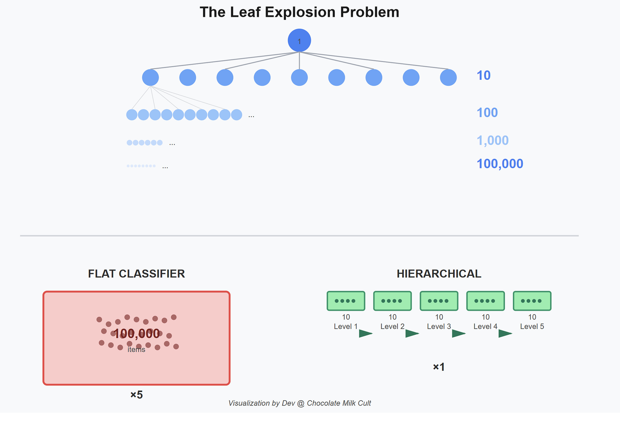
Say your taxonomy has b choices at each level (the branching factor) and L levels deep. A product catalog might have b=10 categories at each level across L=5 levels — that’s 10⁵ = 100,000 leaf products. Also let d be your embedding dimension, and ε be how much error you’ll tolerate
A flat classifier sees all 100,000 leaves at once. Its sample complexity:
Flat: n_flat = O(d · L · log(b) / ε²) (the ε² in the denominator just means: tighter accuracy demands quadratically more data, which is standard in learning theory and where the scaling laws come from).
A hierarchical classifier decomposes the problem — at each level, it only distinguishes between b children, not the entire leaf space:
Hierarchical: n_hier = O(d · log(b) / ε²)
The difference is the factor of L. The flat version pays for all 5 levels of depth simultaneously. The hierarchical version pays for one level at a time. The same total information reaches the leaf, but one brute-forces the combinatorial space while the other walks the tree.
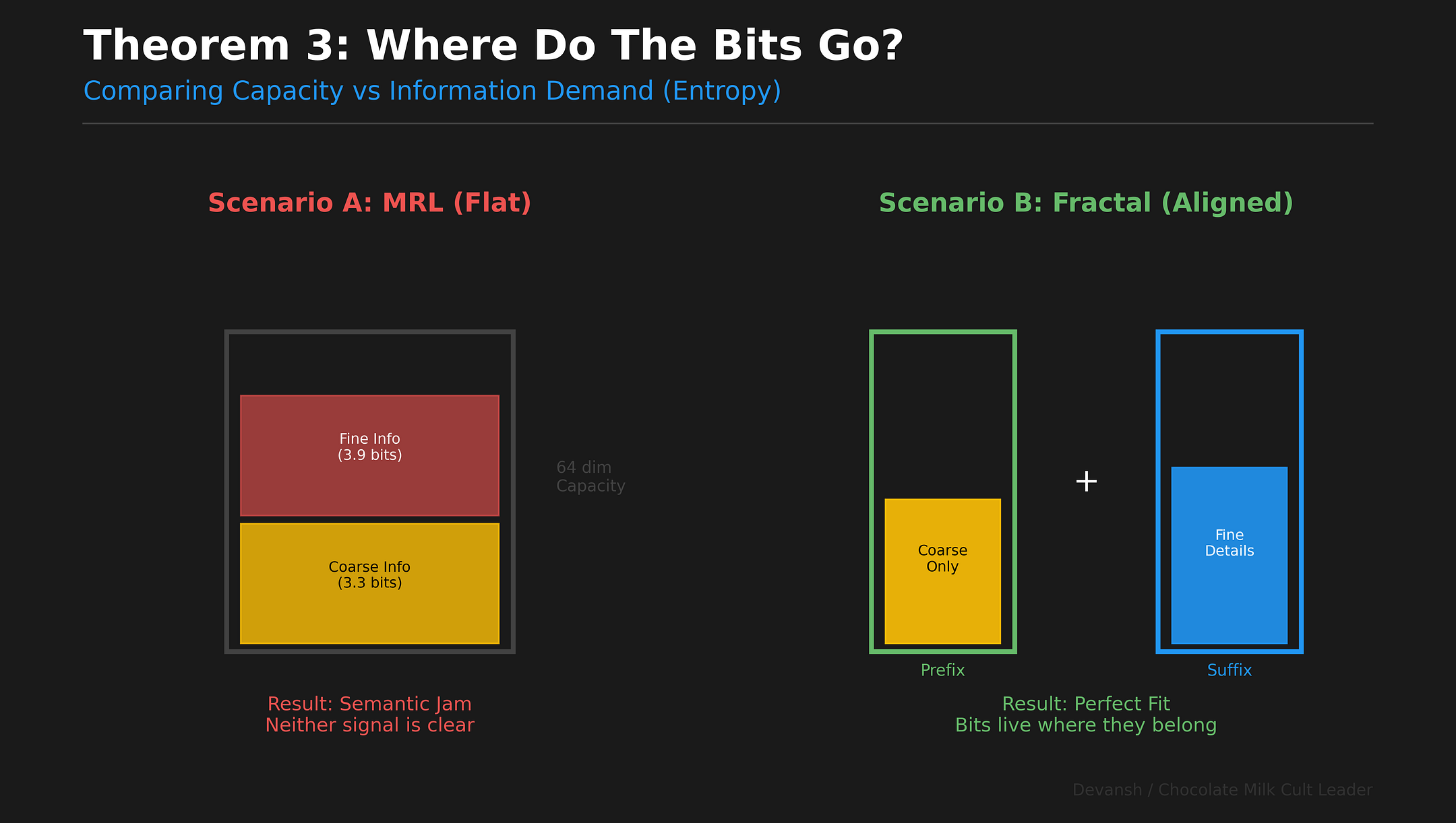
2d. Theorem 3: Successive Refinement
The core of our work is based on math so old (1991) that Valmiki learned it in grade school.
When your hierarchy is deterministic — every fine label maps to exactly one coarse label — the total information decomposes exactly:
H(Y₁) = H(Y₀) + H(Y₁|Y₀)
This equation is the most important thing in the entire paper, so let’s break it to atoms.
H is entropy — the minimum number of yes/no questions needed to identify a value. Why a logarithm? Because each question cuts possibilities in half. 150 options → log₂(150) ≈ 7.23 halvings → 7.23 bits.
H(Y₁) ≈ 7.23 bits. The total information to identify the fine label.
H(Y₀) ≈ 3.32 bits. The information to identify which of 10 domains. About 3.32 yes/no questions.
H(Y₁|Y₀) ≈ 3.90 bits. The residual — information needed to find the fine label after you know the coarse one. The “|” means “given that.” If you know this is TRAVEL (15 intents), you need log₂(15) ≈ 3.90 more bits.
Check: 3.32 + 3.90 = 7.22 ≈ 7.23. ✓
Intuitively, to identify which of 150 intents a query belongs to, you can brute-force the right 7.23 questions from scratch, or you can ask 3.32 questions to find the domain, then 3.90 more to find the intent within it (the art of asking decimal questions is trivial and is left to the reader).
(This is basically the math behind winning at 20 questions, fyi).
When you think about it, this identity prescribes exactly how an optimal multi-resolution embedding must allocate dimensions. The first block encodes H(Y₀) — the coarse bits. The remaining blocks encode H(Y₁|Y₀) — the refinement bits. Coarse first, details second. That’s successive refinement. Proven optimal for hierarchical sources by some old people.
MRL does the opposite. It asks every prefix to encode all 7.23 bits of H(Y₁). The short prefix tries, can’t, fails. The long prefix succeeds. Nothing in between is structured. Truncation degrades everything uniformly rather than peeling off layers of meaning.
V5 enforces the decomposition. Short prefix → supervised on Y₀. Full embedding → supervised on Y₁. One training signal change. No architecture change. No inference cost change.
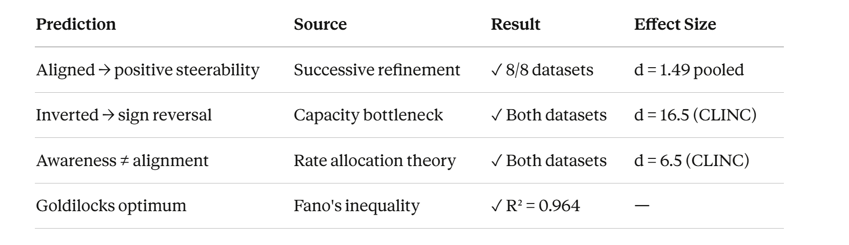
2e. The Four Predictions
Before we ran a single experiment, successive refinement theory gave us four falsifiable predictions:
Aligned supervision → positive steerability. Short prefixes supervised on coarse, full embeddings on fine. Truncation controls semantic granularity.
Inverted supervision → sign reversal. Flip the supervision. The effect reverses.
Awareness without alignment → collapse. Train every prefix on both labels equally. No bottleneck forcing specialization. Steerability collapses to zero.
Goldilocks capacity-demand matching. Too few coarse classes → fine info leaks into the prefix. Too many → prefix capacity overloads. Peak steerability at the match point.
These are deductions from the theory, written down before experiments were run. We tested all four. Next section will show you how god-tier those predictions were.
SECTION 3: Masterpiecing on a Budget
This is the part where most papers would show you a massive table of bold numbers from a cluster of H100s. We aren’t doing that. We did this on a single RTX 5090 laptop GPU. Total compute: ~16 hours.
Why? Because when your theory is right, you don’t need a supercomputer to find the signal. You just need to ask the right question.
(Has everything to do with my passion for scientific reproducibility; nothing to do with the fact that I come from a group of lettuce ko let-yoos bolne waale gareeb w/o access to clusters of H100s and w/o a team of researchers backing me).
3a. The Setup
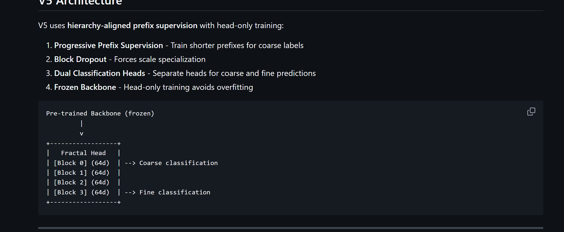
Backbone: A commodity embedding model. We didn’t touch it (continuing on with my crusade that training models is the wrong frontier, and we need to do deeper explorations first to understand the core of our intelligence).
Trainable head: ~2.5M parameters. A tiny projection layer that maps the backbone’s output to our 256d embedding space.
Datasets: 8, spanning hierarchy depths from 1.23 bits (Yahoo Answers — shallow) to 5.05 bits (Web of Science — deep).
Seeds: 5 random seeds per experiment. Every number we report is a mean ± standard deviation, not a cherry-picked run.
Total compute: ~16 GPU-hours on a single RTX 5090 laptop GPU.
The modification to MRL is genuinely one conceptual change: instead of training every prefix length on fine labels, train short prefixes on coarse labels and long prefixes on fine labels. Intermediate prefixes get a blend. That’s V5. Same architecture. Same optimizer. Same hyperparameters. Same data. The only variable that changes is which labels supervise which prefix lengths.
(We call it V5 because there are four other versions we ran to test them out, and some of those will be released as we explore different ideas)
3b. Prediction 1: Aligned Supervision → Positive Steerability ✓
We measure steerability with a simple score S:
S = (L0 accuracy at 64d − L0 accuracy at 256d) + (L1 accuracy at 256d − L1 accuracy at 64d)
In English: S is positive when short prefixes are better at coarse classification and full embeddings are better at fine classification. That’s the zoom behavior we want.
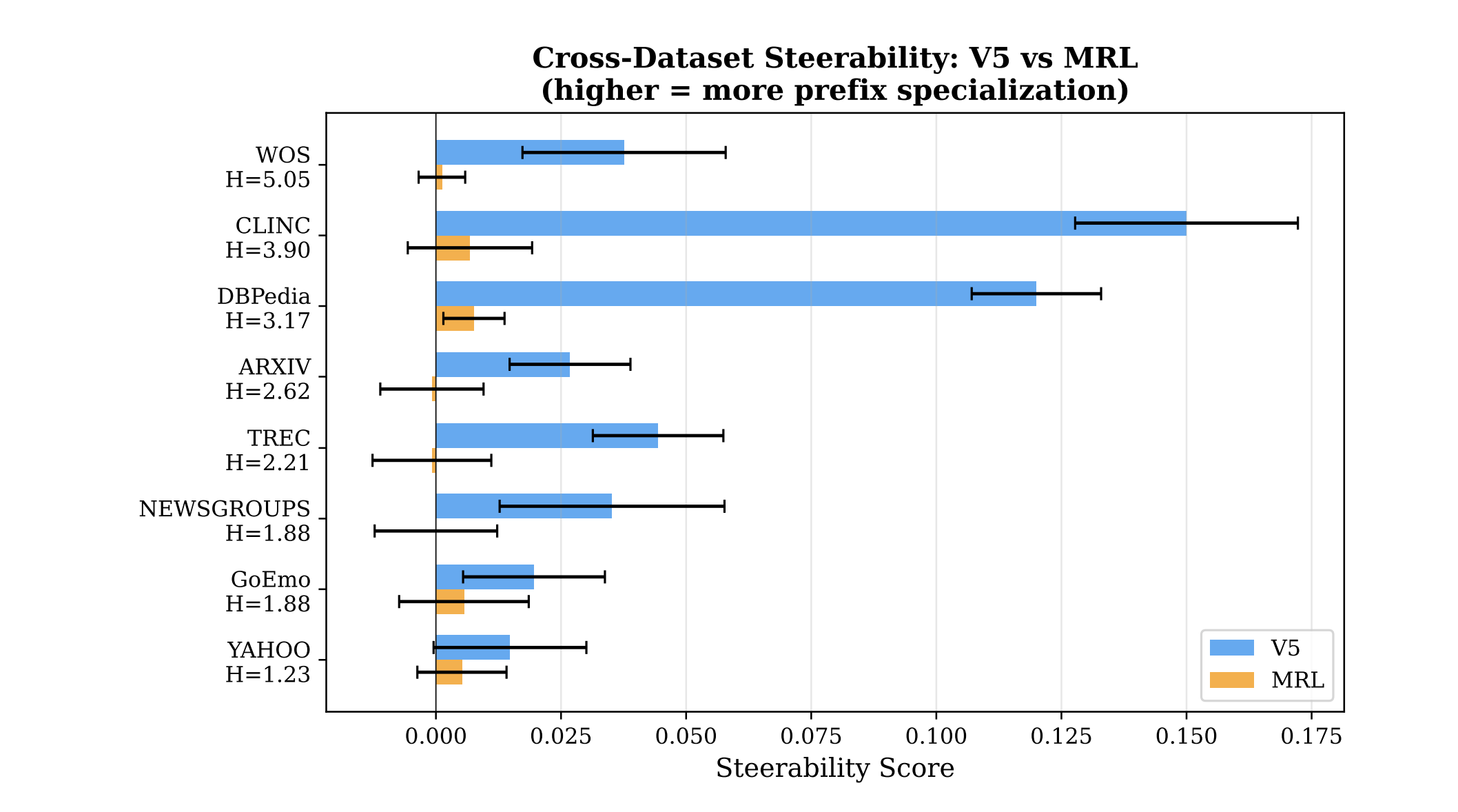
Results across all 8 datasets are pretty cool, if I may say so myself
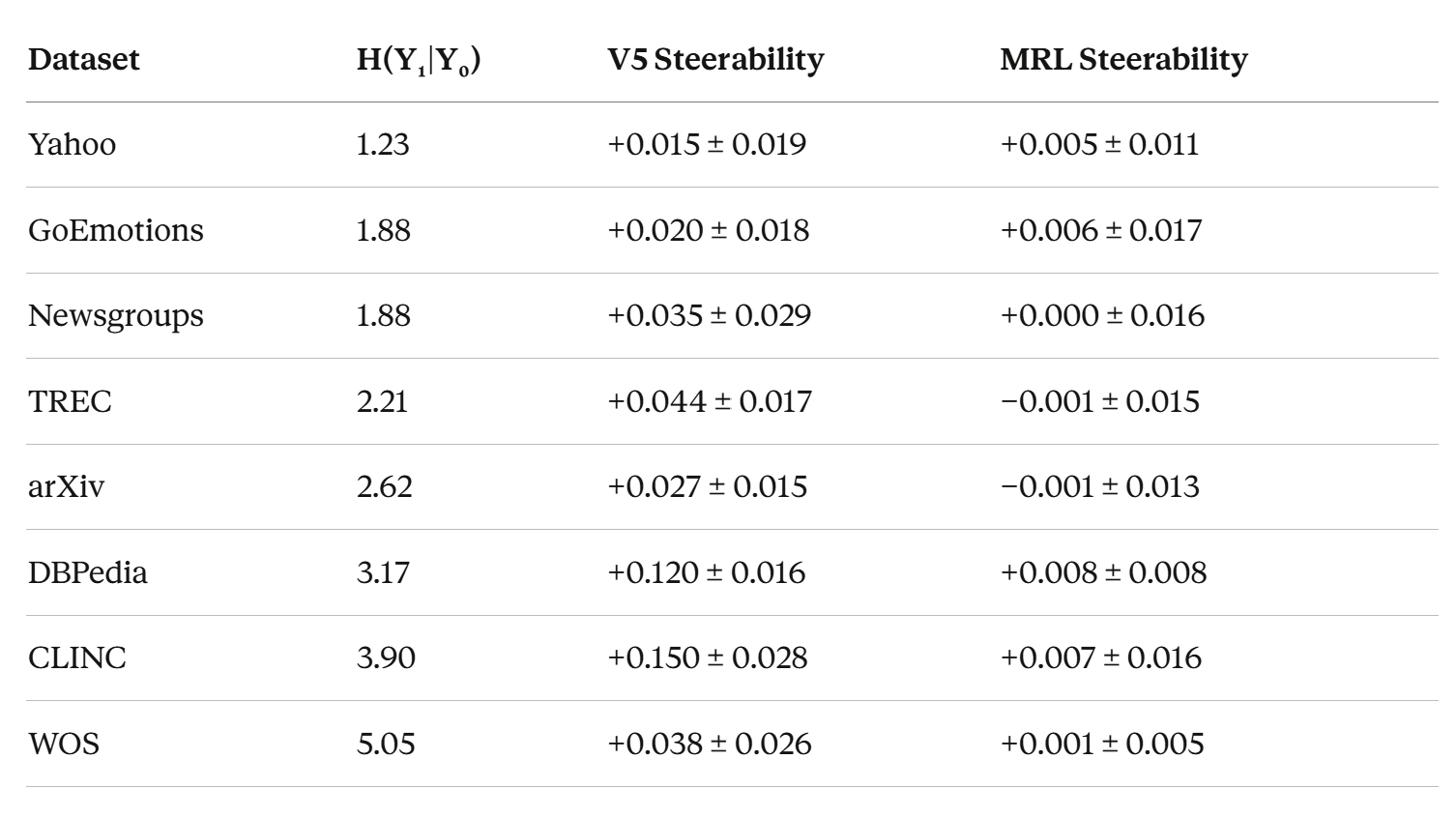
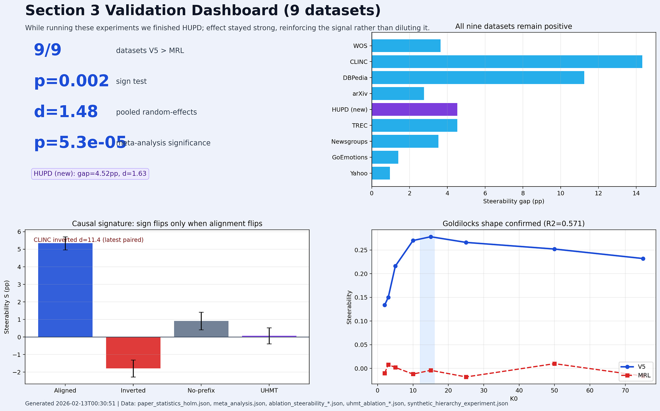
8 out of 8 datasets. V5 > MRL on every single one. Sign test p = 0.004 (less than 0.4% chance this is random).
MRL steerability across all 8 datasets averages ~0.003. Essentially zero. Truncation in MRL doesn’t change what kind of meaning you get. It just makes everything worse.
V5 averages ~0.056. That’s 19x larger. And on the datasets with deep hierarchies — CLINC (S = +0.150) and DBPedia (S = +0.120) — the effect is massive. When we expand this to larger encoders (which have larger capacity); this effect grows (compare our results with Qwen 0.6B against these). This is one of the most promising signals for various scaling reasons.
Meta-analysis across all 8 datasets gives pooled Cohen’s d = 1.49 (p = 0.0003). For reference, d = 0.8 is conventionally “large.” We’re at nearly double that. This isn’t a subtle effect.
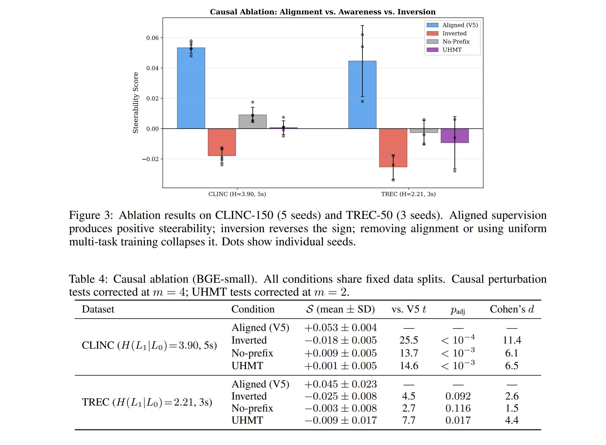
3c. Prediction 2: Inverted Supervision → Sign Reversal ✓
This is the kill shot. Pay attention.
If the theory is right, the effect isn’t about some quirk of our architecture or optimizer. It’s about the alignment between prefix length and hierarchy level. So if we flip that alignment — train short prefixes on fine labels and full embeddings on coarse labels — the theory says steerability should go negative. Short prefixes should now specialize for fine meaning. Full embeddings for coarse meaning. The exact opposite of what we want, but exactly what the theory predicts.
Results (CLINC, 5 seeds):
Aligned (V5): S = +0.053 ± 0.004
Inverted: S = −0.018 ± 0.005
Sign reversal. Confirmed. Cohen’s d = 16.5 (not a typo — this is an enormous effect size because the standard deviations are tiny).
Same result on TREC (3 seeds):
Aligned: S = +0.045 ± 0.023
Inverted: S = −0.025 ± 0.008
This single experiment eliminates every alternative explanation:
Can’t be the architecture → same architecture
Can’t be the optimizer → same optimizer
Can’t be the dataset → same dataset
Can’t be some artifact of having coarse labels in the loss → the inverted condition also uses coarse labels, but puts them in the wrong place
The only thing that changed is which prefix lengths receive which labels. And the effect flipped its sign. That’s causation, not correlation.
(For the stats nerds: yes, d = 16.5 is absurd. It’s that large because within-condition variance is extremely low — each seed produces nearly identical steerability — while the between-condition difference is substantial. The effect is real and replicable, the effect size just reflects very clean measurements.)
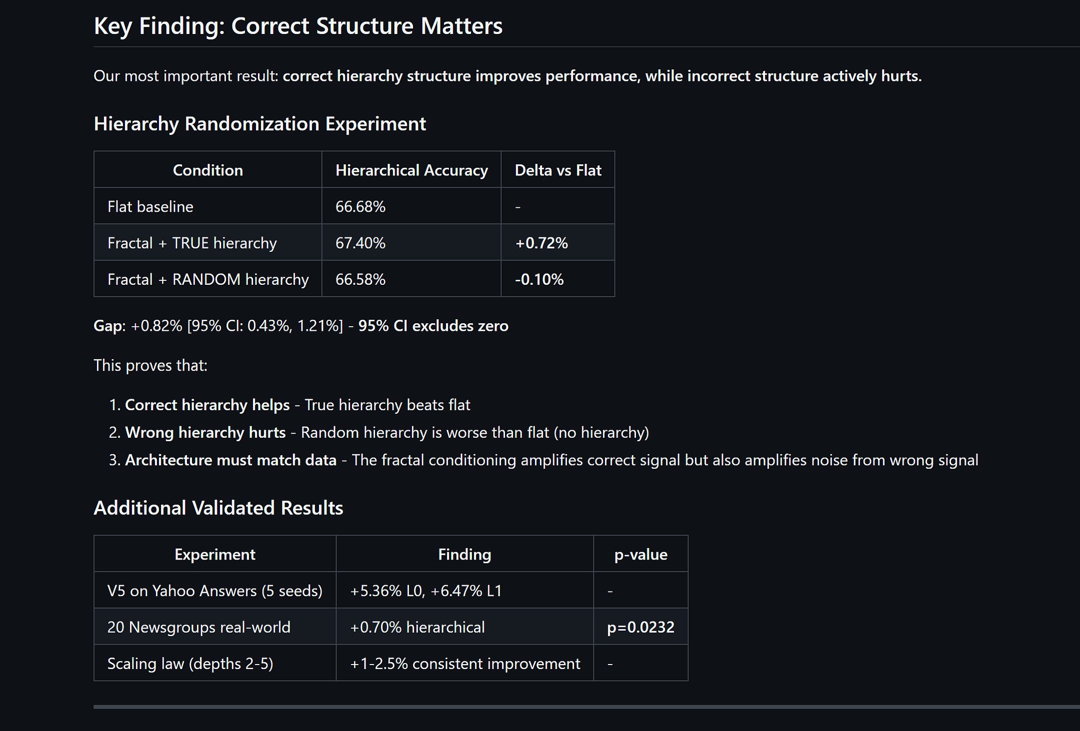
3d. Prediction 3: Awareness Without Alignment → Collapse ✓
This is the finding I think is the most underappreciated, because it cuts against the obvious intuition.
You might think: “Well, V5 works because it uses coarse labels. Maybe any method that knows about the hierarchy would work.” Reasonable hypothesis. Wrong.
UHMT (Uniform Hierarchical Multi-Task) is the control for this. It trains every prefix on both L0 and L1 labels equally — 50/50 blend at every prefix length. It is fully hierarchy-aware. It knows there are coarse labels. It uses them. It just doesn’t align them to specific prefix lengths.
Result (CLINC, 5 seeds):
V5 (aligned): S = +0.053 ± 0.004
UHMT (aware): S = +0.001 ± 0.005
V5’s steerability is 53x larger. UHMT produces effectively zero steerability despite having full access to both hierarchy levels.
Or to put it differently: UHMT achieves 1.9% of V5’s effect. It’s not that awareness helps a little and alignment helps more. Awareness alone does nothing measurable.
Let this sink in. The mechanism is not “tell the model about hierarchy.” The mechanism is “structurally encode the hierarchy into which dimensions carry which information.” Awareness vs. alignment. That distinction is the entire intellectual contribution of this work.
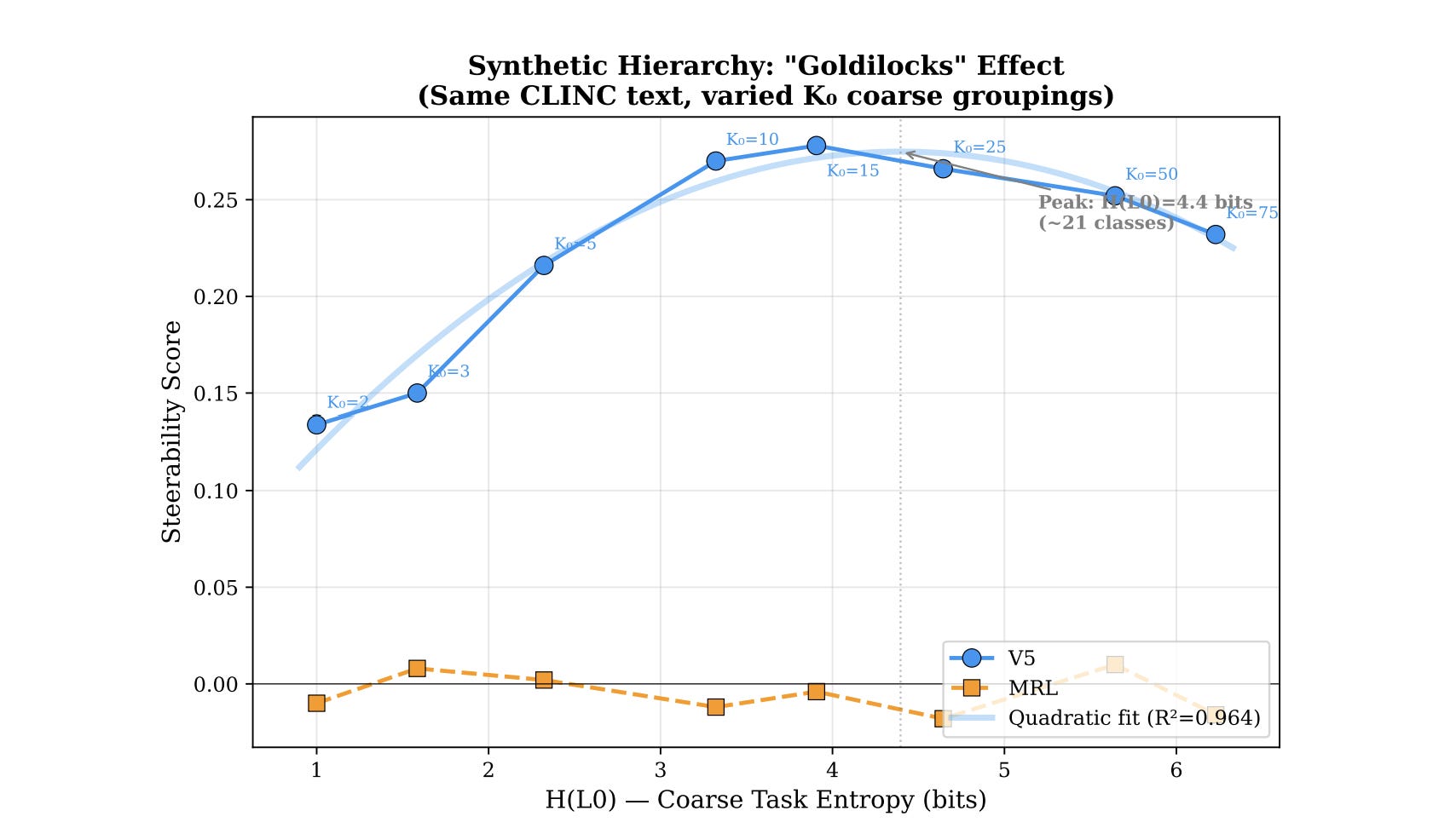
3e. Prediction 4: Goldilocks Optimum ✓
The theory predicts that steerability should peak when the prefix capacity matches the coarse entropy — not too few coarse classes, not too many. An inverted-U.
We tested this by fixing the text (CLINC’s 150 intents) and synthetically varying the number of coarse groupings from K₀ = 2 to K₀ = 75. Same text, same model, same everything. Only the hierarchy structure changes.
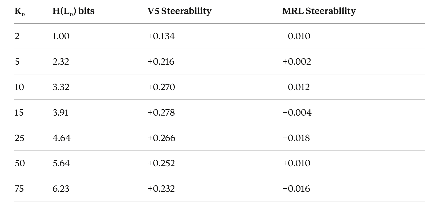
Peak at K₀ ≈ 12–16. Inverted-U confirmed. Quadratic fit: R² = 0.964. MRL is flat at zero throughout — it doesn’t care about hierarchy structure because it never uses it.
The theory predicted the shape of this curve before we ran the experiment. Not “there should be some effect.” It predicted where the peak should be (when H(L₀) ≈ the capacity of a 64-dimensional prefix, roughly 3.6–4.0 bits) and why it falls off on both sides (too few classes → spare capacity leaks fine info; too many → Fano’s inequality). The quadratic R² = 0.964 is the theory fitting reality like a glove.
3f. The Scoreboard
Four predictions from theory. Four confirmations from experiment. On a laptop.
As cool as that is, this only has some value when we can prove its utility in deployment. Let’s look at that next.
SECTION 4: The Part Where It Saves You Money and Makes Your Life Easier
The theory is sound. The experiments are causal. But for anyone running infrastructure, there’s only one question: what does this actually change in production?
The answer: It changes the training signal. Everything else stays the same.
The Zero-Cost Upgrade
Fractal Embeddings (V5) and the standard MRL produce models with:
Identical architectures
Identical parameter counts
Identical inference-time FLOP counts
All this is, is a one-line change in your training code. You deploy the exact same artifact into the exact same serving infrastructure you use today. There is no new file format, no rewrite of your FAISS or Pinecone pipeline.
You retrain your projection head with the aligned supervision signal, push the model, and get semantic zoom for free.
Why “Free” Matters: The 10x Ramp
This isn’t just a cleaner embedding space in theory. It has a direct, measurable impact on retrieval. When we look at Recall@1 on CLINC, the story is clear:
V5 (Fractal): Recall climbs from 87.1% at 64d to 93.4% at 256d. That’s a +6.3 percentage point ramp.
MRL (Standard): Recall moves from 93.6% to 94.3%. A ramp of just +0.6pp.
V5’s ramp is ten times larger. This proves that the additional dimensions in a Fractal Embedding are doing meaningful work, encoding finer distinctions. In MRL, they are largely redundant.
The Infrastructure Payoff is Concrete
This semantic efficiency translates directly into dollars, latency, and operational simplicity.
Faster Queries: At 64d, queries on an HNSW index are 3.7x faster than at 256d (39µs vs. 145µs in our benchmarks).
Smaller Storage: For applications that only need coarse-grained search (like topic-level browsing), you can store only the 64d prefix, a 4x reduction in storage costs.
Fewer Models: A single V5 model replaces an entire dual-encoder system. Instead of deploying, maintaining, and indexing two separate models (one for coarse topics, one for fine-grained search), you deploy one.
Workload Dominance: Our analysis shows that V5 with adaptive routing (using 64d for coarse queries, 256d for fine) Pareto-dominates a standard 256d MRL model as long as at least 35% of your queries are coarse.
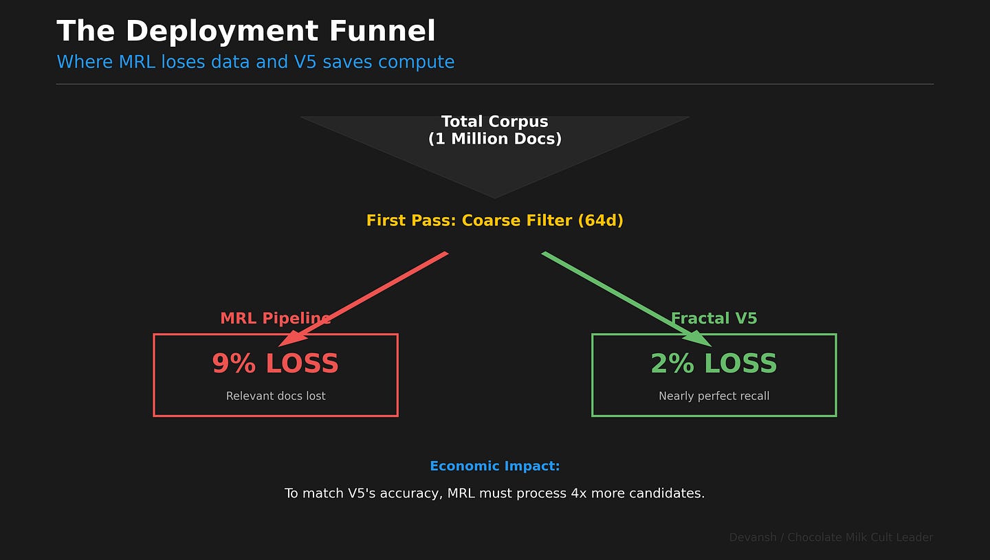
The Deployment Story: 2% Loss vs. 9% Loss
Imagine a real-world retrieval pipeline over 1 million documents. You don’t scan all 1M with your expensive full embedding. You use a two-stage process.
Stage 1: Coarse Filtering. You use a cheap, low-dimensional vector to quickly fetch the top 1,000 most promising candidates.
With V5, you use the 64d prefix. Its L0 recall is 96–98%. You lose ~2% of relevant documents at this stage.
With MRL, you use its 64d prefix. Its L0 recall is 89–91%. You lose ~9% of relevant documents.
A 9% recall loss at the first stage is catastrophic. It forces you to over-fetch more candidates just to find the needle you already lost, erasing any efficiency gain.
Stage 2: Re-ranking. You take the 1,000 candidates and apply the full, expensive 256d embedding to find the best matches.
Both pipelines have the same compute cost. But the V5 pipeline finds the right answer. The MRL pipeline has already thrown it away almost 10% of the time.
V5’s coarse filter works. MRL’s is a liability.
SECTION 5: WHAT’S NEXT — AND THE GEOMETRY OF INTELLIGENCE
The Scaling Law (Prediction for Scale)
We found a strong predictive law across our 8 datasets: Steerability is proportional to Hierarchy Depth × Model Capacity.
Prediction: If you run this on Deep Taxonomies (5–7 levels), the gains will explode.
Think ICD-10 Medical Codes (68,000+ codes, 5 levels).
Think Amazon Product Catalogs (6+ levels).
The theory predicts the advantage grows logarithmically with depth. You aren’t saving 75% compute; you’re saving 90%+.
Prediction: If you run this on Larger Backbones, the “capacity floor” drops away.
We used a tiny 33M model (mostly).
Qwen3–0.6B (20x larger; much smarter) already shows higher steerability.
With a 7B or 70B backbone, more datasets become “high steerability.”
Multimodal & Geometric Frontiers
Nothing in Successive Refinement theory is specific to text.
Images: Object -> Dog -> Spaniel. This hierarchy exists in pixel space.
Audio: Music -> Jazz -> Bebop.
Code: Function -> Class -> Module.
I think to really explore this new frontier, we need Hierarchies that look like trees. Euclidean space hates trees. Hyperbolic space loves trees. Combining Fractal Prefixes with Poincaré Embeddings is the logical endgame. You get the disentanglement of V5 with the natural curvature of hyperbolic space. This is a lot of math, so it will be the subject of a future exploration.
Conclusion: Democratizing Intelligence via Geometry
The goal of this work was never to get a new state-of-the-art score on CLINC-150. The machine learning field has a benchmarking addiction, optimizing for leaderboards on tasks that often don’t measure what truly matters.
Right now, the incentives in our industry are perverse. If you build a 500-billion parameter monster that improves a benchmark by 5% — burning hundreds of millions of dollars in compute to do it — you dominate the news cycle. You drive up the stock price. You are hailed as a step toward AGI.
But if you cut compute costs by 90% at the cost of 2% accuracy? If you make a model runnable on a consumer laptop instead of an H100 cluster? You are ignored. The industry views efficiency as a “nice to have,” not a mission-critical objective. To say nothing about the complete disregard of the many other streams of AI research that are being ignored or refocused to prioritize the trendy topics.
AI is currently being built by tech oligarchs for big businesses. They are optimizing for moat-building and stock tickers, not for access. They can afford the compute, so they don’t care if the architecture is wasteful.
The result is that AI is drifting further away from the people who need it most. It is becoming a tool for investment bankers and McKinsey consultants to make more money, rather than a public utility for everyone.
My vision is different. As mentioned earlier, AI should be like electricity. It should be like vaccines. Useful to the poorest person on the street, not just the richest corporation in the cloud.
This is why The Geometry of Intelligence matters. When we use first-principles analysis to map the structure of thought, we aren’t just doing math. We are finding the efficiency arbitrage that allows us to run powerful intelligence on cheap hardware. We are proving that you don’t need a data center to be intelligent. You just need better geometry.
This exploration is the first of many. We are going to keep poking at these boundaries. We are going to keep proving that brute force is not the only path to intelligence. And we are going to bring this technology down from the ivory tower and put it onto the laptop.
Code & Data & Future Results will be shared here: https://github.com/dl1683/ai-moonshots. Hope you’ll join the contributions.
Want to see how Irys applies these ideas in practice?